|
The ABC Study Guide, University education in plain English alphabetically indexed. Click here to go to the main index |

|

|
|
ABC StatisticsStatistics is the study of large numbers, such as those produced by government departments, with the aim of extracting some approximate truth from them.There are descriptive statistics and inferential statistics
|
Statistics: Origin and Meaning
One of the origins of statistics origins is state arithmetic
- "The word Statistics appears to have been first used about the middle
of the last [18th] century by Achenwall, a professor at
Gottingen, to
express a summary view of the physical, moral, and political condition of
states".
(Hawkins, F. B.
1829 p.1)
- "The word Statistics is of German origin, and is derived from the word
staat, signifying the same as our English word state, or a
body of men existing in social union. Statistics, therefore, may be said,
in the words of the Prospectus of this society, to be the ascertaining and
bringing together of those "facts which are calculated to illustrate the
condition and prospects of society;" and the objects of Statistical Science
is to consider the results which they produce, with a view to determine
those principles upon which the well being of society depends. Journal
of the
Statistical Society of London
May
1838. Vol.1, No.1,
Introduction.
"The Science of Statistics differs from Political Economy, because, although it has the same end in view, it does not discuss causes, nor reason upon probable effects; it seeks only to collect, arrange, and compare, that class of facts which alone can form the basis of correct conclusions with respect to social and political government". Journal of the Statistical Society of London May 1838. Vol.1, No.1, Introduction.
History of statistics: Roman census - 1086 - Probability - John Graunt - 1710 - Scotland's statistical account - 1801 British census - the begining of crime statistics - Benjamin Gompertz - British Association - 1833: Statistical Societies formed - Quetelet's average person - 1837: births, deaths and marriages - objective statistics - 1841 British census - suicide statistics - 1857: Henry Thomas Buckle - Alexander von Oettingen - 1878?: cycles and sunspots - Enrico Morselli on suicide statistics - Charles Booth - 1913: Class - 1922 Fisher: Mathematical Foundations - 1927: Carr-Saunders and Caradog Jones social structure statistics - Wartime Social Survey - 1960s: computers and statistics - Statistical Package for the Social Sciences - 1970: Office of Population Censuses and Surveys - 1976: Radical statistics - 1992: UK Cochrane Centre - 1997: UN Official Statistics Principles - 1996: Office for National Statistics - 2013: International Year of Statistics
Descriptive
Statistics
Descriptive statistics allow us to describe
groups
of many numbers. One
way to do this is by reducing them to a few numbers that are typical of the
groups, or describe their characteristics. The
average
is one kind of
descriptive statistic. Measures of
spread
are another
kind.
Grouping numbers into
frequency
distributions
and drawing
charts
to
illustrate frequency distributions, are other examples of descriptive
statistics.
Inferential
Statistics
,
Statistical Tests or
Inductive Statistics
Inferential statistics do not just describe numbers, they infer causes.
We use them to draw inferences (informed guesses) about situations where we
have only gathered part of the information that exists. The part of the
information is called a
sample.
The whole body of information from which it
is taken is called the
population.
In a basic
statistical test we would have two samples and would try to establish if
they are
significantly
different.
Statistical inference is the use of samples to reach conclusions about
the population from which those samples have been drawn.
For example, twenty people who have not read this passage would be one
sample. The same twenty people after they
have read the passage is another sample. The population from which both
samples are drawn is all the people who could (in theory) read this
passage. If we found that,
- before reading this passage, many of the twenty people could explain
what inferential statistics is.
- after reading this passage, none of the twenty people could explain what inferential statistics is.
Statistical analysis refers to doing something useful with data
(letting its
meaning free).
The two main
ways that data is analysed are:
- by bringing out the information it contains. This is part of
descriptive statistics
- testing or retesting a hypothesis. Hypothesis testing is part of inferential statistics.
 Advice about Statistical Analysis
The different meanings of analysis
Advice about Statistical Analysis
The different meanings of analysis
Primary analysis is the original analysis of data in a research study.
Secondary analysis is the re-analyis of data. This could be to answer new questions or to use improved statistical techniques,
meta-analyis is the statistical analysis of a large collection of analysis results to integrate the findings.
Dataset A collection of data. For example:
{2, 3, 5, 8, 12}
Raw Data
Statistical lies
Wikipedia:
Lies, damned lies, and statistics
How to lie and cheat with statistics
A Census is an official counting of
people (or sometimes things)
in a state or other political area. It is one of the oldest, and most
important, forms of
descriptive statistics.
Estimates of the
Chinese population relate to all the dynasties, but the first
"tolerably accurate" census of China is said to be that of
AD 2.
(Hollingsworth T. H. 1969 pp 65-66 and 67)
The
birth of Christ
is said to have taken place in Bethlehem because of a Roman census.
The regular ten year census of all the British population began in
1801
See
Office for National Statistics for some publications
A Combination is the selection of a number of items from a
larger number in which the order of selection does not matter.
For example, if we have five items, how many ways can we select three
from the five if we are not bothered about what order the items appear in?
We will call the five items A,B,C,D,E
We can now set them out to show that there are ten ways in which they
can be combined in groups of three:
ABC ABD ABE
A Permutation is the selection of a number of items from a
larger number when the order the items appears in does matter.
For example, ABC, ACB, BAC, BCA, CAB and CBA are all the same
combination, because they contain the same three items, but they are
six different permutations, because the items are in a different
order.
Control Group
A scientific control group is a group that is matched with an
experimental group on everything believed relevant - except the thing to be
tested.
William Farr
used the patients in
Gloucester County Asylum as his control group when trying to find out if
the death rate in London madhouses was abnormally high.
This illustrates one of the reasons for a control group. Farr could not
could not say if there was anything abnormal about a high death rate in
London madhouses unless he could show it lower in another asylum.
If you were trying to show that criminals come from broken-homes, you would
need a control group of non-criminals to compare. If 20% of criminals came
from broken homes and 25% of non-criminals, you could not argue (on the
basis of those statistics) that broken homes are a cause of criminal
behaviour.
An experiment or trial that uses a control group is a controlled
one. In medical research a controlled trial is one where one group
of participants receives an experimental drug while the other receives
either a placebo (a substance containing no medication) or standard
treatment. See the
example of text massaging.
Blinding is hiding from participants which group they are in.
Observer-blind is when the researcher does not know the groups.
Single-blind is when only the participants do not know which group they are
in. Double-blind is when both the participants and the researcher
do not know group identity. Blinding is engaged in to protect
results from bias.
Andrew Weil, Norman Zinberg and Judith Nelson'
"controlled
experiment on the effects of marihuana" (1968) has been
described as comparing "the effects of
smoking the drug on a series of naive subjects contrasting them with a
control group of chronic users". However, each group was given a placebo at
some sessions and the real thing at others. Weil, Zinberg and Nelson appear
to have regarded this as the control.
Correlation
If two things correlate, one changes in relation to changes in the other.
The change can be positive or negative. For example, the height of a pile
of coins increases as extra coins are added (positive correlation). On the
other hand, pain may decrease with an increase in pain killer (negative
correlation)
Correlation is a measure of the association between the two things that
change (the
variables). The closer to 1 means a stronger positive
correlation. The closer to -1 means a stronger negative correlation
Population
In
statistics,
population does not
necessarily mean
people. It is a technical term for the whole
group
of
people or objects the results apply to. In a statistical survey of London
pigeons, the population is all the pigeons in London. As there are a lot of
pigeons in London, a statistician would take a
sample
rather than inspecting every one.
If you toss a coin into the air it can land on one of two sides
Probability is measured on a scale going from 0 for an absolute
impossibility to 1 for an absolute certainty.
I never buy lottery tickets so:
In coin tossing, the probabilities of different outcomes can be worked out
using a
binomial probability calculator
Toss a well-balanced coin once and the probability of heads is 0.5. and the
probability of tails is 0.5.
Bernoulli trials - Binomial distribution - normal
cuve
Random: See
sample and
probability sample
Regression to the
mean is a movement of figures towards an
average.
Galton's large and small sweet pea seeds, for example, gave rise
to plants with more averages size seeds.
The exploration of relationships between
variables
is called regression
analysis or regression modelling.
Correlation and regression both attempt to describe the
association between
two (or more) variables, but only regression assumes that one variable (x)
causes the changes in the other (y)
Leicester explains the difference between correlation and regression
Sample and example
Example and sample originally meant more or less the same. A sample was a
particular incident or story that was supposed to support a general
statement. An example was a typical fact that illustrated a general
statement. The difficulty of making a fair "sample" in this sense are
obvious. We would not (I hope) accept "all men are nasty - take Hitler" as
conclusive proof.
Sample in statistics:
A
statistical
sample is a selection of part
of a
population
chosen to provide information
about the whole population. To do this, a sample needs to be
representative
(or not unrepresentative) of the population (the universe from which it is
supposed to be drawn).
Julie Ford explains this by saying
If you are researching the feelings of sociology students (generally) about
mathematics, your sample would be unrepresentative if it was
exclusively
drawn from the membership of an optional maths for sociologists class as
those students have actually chosen to study mathematics. You might,
however, use such a sample and compare it with a sample of students who had
chosen to join a class on
qualitative methods. This would be an example of
purposive sample.
If, on the other hand, you selected a sample from all sociology students
taken at random, it would be a
probability sample.
A probability sampling method is any
method of sampling that utilizes some form of random selection.
A random sample is one where any item in the population was as
likely as any other to be in the sample, and where the selection of one
item did not affect the selection of any other. In everyday life people try
to make random samples by putting tickets in a hat, shaking them up, and
then asking someone to pick a few out without looking into the hat. Random
samples are made by blind chance.
Probability sampling can draw on
probability theory to assess how
representative of the
population they are.
Nonprobability sampling does not involve random selection. Two broad
categories of nonprobability sampling are
purposive sampling and
convenience sampling
A purposive
sample is one where the sample is selected because it is
thought to be representative in some way.
A purposive sample may be selected on the basis that the units are the same
(homogeneneous) or different (heterogeneous).
Julie Ford gives as examples
the selection of samples to test a
hypothesis about
eating and obesity.
Eating might be the cause of fatness, but how would one control for the
effect of exercise? One way would be to select a sample of people who do
about the same amount of exercise (a
homogeneneous sample). Another way
would be to select range of samples of people with different
(heterogeneous)
exercise habits. One sample might be people who did a lot
of exercise, another medium exercisers and another low exercisers. In this
case, comparisons could be made between the samples.
(Ford 1975 p.266).
Julie Ford calls heterogeneous samples, such as the above,
examples of typological sampling
Another method is matching samples, which combines homogeneous and
hterogeneous sampling
Structural sampling or Quota sampling
Julie Ford's example of organising samples by the academic year of a school
for young gentlewoman, and the knicker wearing habits of the young ladies,
belongs to the age of innocence, before the
exposure of Jimmy Savile
An opportunity sample is one where the sample is selected because it
is convenient for the researcher. Interviewees, for example, might
be
selected because they are easily accessible, willing to participate and
available at a convenient time. An example would be a student researcher
using fellow students to interview. Has also been called an incidental
sample, a convenience sample, a haphazard sample and an
accidental sample
Snowball sampling
See
diagram
Spread, or dispersion, refers to how far out our figures go. A chunk of
butter on a slice of bread is hardly spread at all. The same chunk can be
spread out thickly or thinly. The larger area it covers, he more its
spread. It is the same with figures.
The first
array of figures is thinly spread:
1, 1, 2, 2, 2, 3, 3, 3, 3, 4, 4, 4, 4, 4, 5, 5, 5, 5, 5, 5, 6, 6, 6, 6, 6,
7, 7, 7, 7, 8, 8, 8, 9, 9
The second
array of figures is thickly spread:
4, 4, 4, 4, 4, 4, 4, 4, 4, 4, 4, 5, 5, 5, 5, 5, 5, 5, 5, 5, 5, 5, 5, 6, 6,
6, 6, 6, 6, 6, 6, 6, 6, 6
Nevertheless, the
averages of the figures are the same: The
arithmetical mean is
170, the
median and the
mode are both 5.
The standard deviation is a measure of how
spread out a
dataset is.
It tells us how far items in the
dataset are, on
average, from the
mean.
The larger the Standard Deviation, the more
spread out the data are.
For the dataset {2, 3, 5, 8, 12} the mean is 6. So
the deviations from the mean are {-4, -3, -1, 2, 6}. We square these
deviations, {16, 9, 1, 4, 36}, and take their average, 13.2. Finally we
take the
square root of 13.2 to give us the Standard Deviation, 3.63.
Some of the
statistics with the oldest history are figures year by year (or
some other period) showing how something has changed. These are time
series. Examples are
balance of trade series -
crime series and
suicides
series. The time series you will see by clicking the above links
are composed of
absolute figures, but
time series may also be composed of
ratios
Andrew Roberts likes to hear from users:
Statistical
Data
The raw data of statistics is groups of numbers that the statistician
intends to work on. They are the numbers before they have been organised
and processed.
For example:
6, 6, 7, 9, 3, 4, 4, 7, 2, 3, 8, 5, 6, 6, 7, 1, 2, 3, 1, 7, 3, 4, 8, 5,
5, 8, 2, 9, 5, 4, 4, 5, 6, 5
Array
In mathematics, an array is an arrangement of numbers or
symbols in rows and columns. In statistics it is a group of numbers in rows
and columns with the smallest at the beginning and the rest in order of
size up to the largest at the end.
For example:
1, 1, 2, 2, 2, 3, 3, 3, 3, 4, 4, 4, 4, 4, 5, 5, 5, 5, 5, 5, 6, 6, 6, 6,
6, 7, 7, 7, 7, 8, 8, 8, 9, 9
Frequency Distribution
A frequency distribution is an arrangement of a group of numbers in a
pattern that shows how frequently each occurs. This is done by grouping
(classifying) the numbers and arranging them in a table according to size:
For example:
1, 1
2, 2, 2
3, 3, 3, 3
4, 4, 4, 4, 4
5, 5, 5, 5, 5, 5
6, 6, 6, 6, 6
7, 7, 7, 7
8, 8, 8
9, 9
Statistically Significant
Statistical significance is a way of estimating the likelihood that a
difference between two
samples
indicates a real
difference between the
populations
from which the
samples are taken, rather than being due to
chance.
If a result is very unlikely to have arisen
by chance we say it is statistically significant.
If a result would
only arrive by chance once in a hundred times, we would call it
significant. If only once in 1,000 times, it would be highly
significant. If once in twenty times, only probably significant
Statistical significance is express in terms of
probability.
We say, for example, that:
See
Statistical Experiments
What did Engels mean
by taking the average?
Average: Averages are ways of
describing what is typical,
normal or
usual.
People come
in lots of sizes, but the average adult
is not 8 feet tall or 3 foot small.
How can we measure what the average is? The way that most of us know
for making an average is technically called:
The arithmetic mean. To work out one of these you:
First
add
a group of numbers together
Then
divide
by the number of numbers in the
group.
For example:
The (mean) average of 3, and 8 is the total (11)
divided by the number of numbers (2),
giving 5.5 as the average (arithmetic mean).
The (mean) average of
3, 4, 5, 5, 6, 6, 6, 7 and 8 is the total (50)
divided by the number of numbers (9),
giving 5.55 as the average (arithmetic mean).
Another kind of average is:
The median
Instead of adding the group of numbers together, we arrange them in
order of size from the smallest to the largest. The median is the middle
number.
For example:
The median of
3, 4, 5, 5, 6, 6, 6, 7, 8
is 6
If the number of numbers is even, there will be two middle numbers.
In these cases, the median is the number half-way between the two
middle
numbers.
For example:
The median of 3 and 8 is 5.5
The median of 4, 5, 5, 5, 6, 6, 6, 7 is also 5.5
The median of 1, 2, 3, 4, 5, 6, 7, 8 is 4.5
Another kind of
average
is:
The mode
The mode (or modal number) is the number that occurs most frequently.
For example:
The mode of
3, 4, 5, 5, 6, 6, 6, 7, 8
is 6
If two or more numbers occur the same number of times, and more often
than the other numbers, there is more than one mode.
For example:
The modes of
3, 4, 5, 5, 5, 5.5, 6, 6, 6, 7, 8
are 5 and 6
If each number occurs the same number of time, the group of numbers has
no mode. There is no mode in this group: 3, 3, 4, 4, 5, 5.
Census
Combinations and Permutations
ACD ACE
ADE
BCD BCE
BDE
CDE
Probability
Probability is the chance that something will happen
See
1622 -
1710 -
1713 -
1824 -
1835 -
The probability that it will land on a particular side is 50%, or one
chance in two.
No possibility is written p = 0
One chance in 1,000 is written p = 0.001
One chance in 100 is written p = 0.01
One chance in 20 is written p = 0.05
One chance in 10 is written p = 0.1
One chance in 2 is written p = 0.5
7 chances in 10 is written p = 0.7
99 chances in 10 is written p = 0.99
Absolute certainty is written p = 1
Tossed twice the probability of heads once is 0.5, heads twice is
0.250, and not at all is 0.250
Tossed three times the probability of heads once is 0.3750, twice is
0.3750, three times is 0.1250 and not at all is 0.1250.
See
Randomised Controlled Trial
Looking at the
graph relating Galton's sweet pea sizes, we see that the
relation of the measures of parent and average offspring seeds would be
joined by a wriggly line, but a straight line has been estimated for them
This is called the regression line. It allows a relatively simple
mathematical formula to be given for the relationship.
Chance, Winter 1997, pp 42-45
"An unrepresentative (or biased) sample is one which differs in
relevant respects from the universe from which it is supposed to be drawn"
(Ford 1975 p.265).
"The most popular way of obtaining a structural
purposive sample
is by opting for quantitative of numerical
isomorphism. This is...
the
kind of sampling known as
Quota Sampling... But sociologists have
also devised" [sampling systems that attempt] "to draw a qualitative or
interactional rather than a quantitative
isomorph of the universe in
question. The most commonly used type of interactional sampling is ...
snowball sampling"
(Ford 1975 p.301).
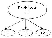
In a snowball sample, one participant leads the researcher on to another
participant.
Spread or Dispersion.
Standard deviation
origin
- variation
- deviance
 Study
links outside this site
Study
links outside this site
 Andrew Roberts' web Study Guide
Picture introduction to this site
Top of
Page
Take a Break - Read a Poem
Andrew Roberts' web Study Guide
Picture introduction to this site
Top of
Page
Take a Break - Read a Poem
 Click coloured words to go where you want
To contact him, please
use the Communication
Form
Maths index
*****************
Statistics index
Blue: this page. Red: other pages. Pink: fairytale